To talk about an introduction to econometrics, it is necessary to establish the mathematical and statistical foundations to understand it. Starting from the summation:

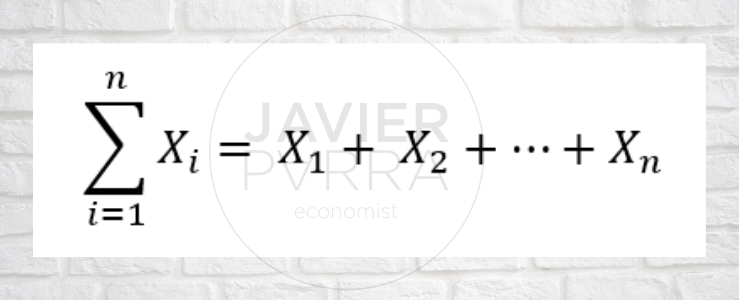
• The symbol Σ is the Greek capital letter sigma and means “the sum of”.
• The letter i is called the summation index; this letter is arbitrary and can also appear as t, j or k.
• The expression ∑(i=1)^n is read as the sum of Xn‘s terms from i equal to one up to n.
• The numbers i and n are the lower bound and upper bound of the summation.

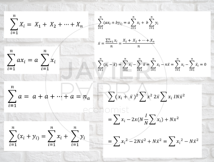
Rules of the addition operation

• A random variable is a variable whose value is unknown until it is observed.
• A discrete random variable can only take a limited or countable number of values.
• A continuous random variable can take any value in an interval.
• The population is the set of individuals who have certain characteristics and are of interest to a researcher.
• The sample is a subset of the population.

Population and sample moments

The sample mean, mean or expected values:

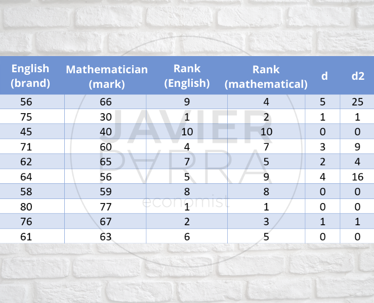
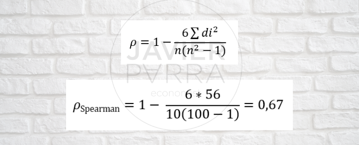
A monotonic relationship is one of the following:

1. When the value of one variable increases, so does the value of the other.
2. When the value of one variable decreases, the value of the other variable decreases.

Let’s look at the following examples of monotonic and non-monotonic relationships:

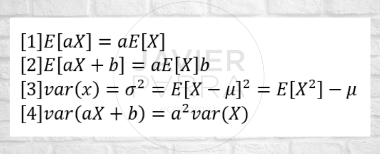
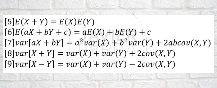
Expected values of the functions of a random variable

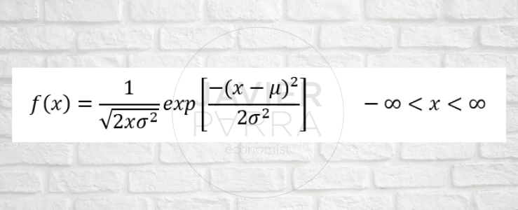
Some important probability distributions

Normal or Gaussian; if X is a normally distributed random variable with mean 𝝻 and variance σ², it can be symbolised as X~N(𝝻,σ²)

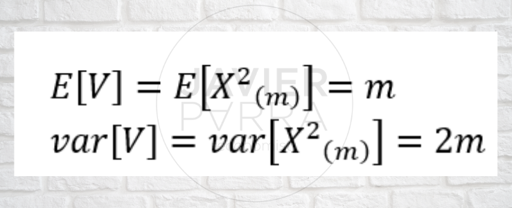
Chi-square: If X, is a normally distributed random variable with mean 0 and variance σ², then V= X₁² +X₂² +…+X_m² ~ X(_m)²

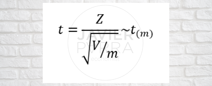
A Student’s random variable is formed by dividing a standard normal random variable with mean 0 and variance 1 by the square root of an independent chi-squared random variable, V, divided by its m degrees of freedom.

No olvides compartir

Facebook

Twitter

Linkedin

Whatsapp